| Prominence Definitions - Error Analysis * |
|
Introduction |
Table of Contents |
Very often exact peak and/or key saddle elevations are unavailable. However their values are generally known to lie within specific topographic map contour intervals. Estimates are then made for the uncertain elevations with the goal of computing prominence (peak minus saddle elevation). Three types of estimates may be applied - clean prominence, interpolated ("mean") prominence and dirty ("optimistic") prominence.
None of these estimation processes are ideal, with the advantages and drawbacks of each having been discussed. In this note error distributions of the reported prominences resulting from these estimates are calculated. It will then be evident that interpolated prominence has overwhelming advantages in a statistical sense. Subsequent treatment is thereby limited to interpolated prominence.
Prominence-based peak lists rely upon these estimates for both ranking peaks and for whether peaks meet the list cutoff criterion at its bottom. Indeed, at a list's end there is a small number of peaks which lie in a "gray zone" wherein their presence or absence is not clear-cut, i.e. it is uncertain whether a given peak truly has a prominence worthy of meeting the prominence list cutoff criterion - and this uncertainty results from the estimation process and measurement errors.1,2 In this note the probabilities of correctly listing or not listing peaks are calculated for all three estimation types at various levels of refinement.3
These issues and their implications are considered here. Then, to perform detailed calculations of error probabilities a new measure arises in a natural fashion which in several aspects is the antithesis of topographic prominence.
1. The expression "gray zone" has not been universally accepted throughout the prominence community.
However its intended meaning should be clear, the color gray lying somewhere between white and black.
Table of Contents
Historically clean prominence was the first definition employed in published prominence-ordered peaklists. The longstanding belief has been that a peak on such a list is guaranteed to meet the list's cutoff prominence value. As such it is presumably an unambiguous list - no subjectivity is involved in deciding whether a peak is to be represented.
This surprising statement (which is surely disconcerting to the clean prominence list preparer) arises because of measurement errors in the peak and saddle elevation contours. Practical arguments and calculated examples are provided later to confirm this statement.
Consider a climber pursuing such a list. The goal, most commonly, is to reach the summit of every peak in the given geographic or political region so represented. Unfortunately the clean list does not suffice - in general there will be peaks that might meet the list cutoff value (henceforth "Pcutoff"), yet do not have the corresponding clean prominence.
This is a problem. To partially address it the list researcher typically inserts a set of footnotes which list all peaks that have an optimistic prominence of at least the list's cutoff value, yet do not have the corresponding clean prominence. The climber, if worth his salt, will attempt to climb these footnoted peaks as well so that he is guaranteed to have climbed every summit which could possibly have at least Pcutoff .
Again, this heretical statement arises due to peak and saddle elevation contour measurement errors.
Enter interpolated prominence. Why use it at all? First, in using the average of possible peak and/or saddle elevations one has the intuitively most unbiased assessment of the resulting prominence, i.e. there is no intentionally harsh underestimate (as with clean prominence), nor is there an intentionally lenient overestimate (as with optimistic prominence).
Indeed, of these three prominence definitions, it is only interpolated prominence that is an unbiased estimator of peak and saddle elevations lying within a range of possible values.4,5 Thereby it provides the most statistically sound estimates for the true (yet currently unknowable) peak prominences. As an importance consequence, as shown later interpolated prominence provides the largest probability that gray zone peaks are correctly displayed (or not displayed) on the corresponding prominence list.
Henceforth clean, interpolated (mean) and optimistic (dirty) prominence are sometimes denoted by Pmin, Pinterp and Pmax, respectively.
Invariably a prominence-based peak list contains entries of varying accuracy. The majority of saddle elevations will only be known to within a map contour interval. Some peaks will have spot elevations while others will not. Thereby the rank ordering of peaks varies depending on which prominence definition generates the list since the numerical differences between computed clean, interpolated and optimistic prominence for a given peak depend upon how accurately its elevation is known - and that of its key saddle. Thus when the accuracy varies so do these differences - and adjacently-listed peak's relative ranks often switch places from one list to the next simply because the authors have selected different prominence definitions.
This is a confusing state of affairs to the reader. If every published list were to have peaks ranked according to, for instance, mean prominence the problem would vanish.
There are lists of the N most prominent peaks in a specified region, e.g. the North America Fifty Finest.6 Near the list's bottom may be a few peaks that "compete" for the last few positions. There might be four such mountains and only two remaining slots on the list - ranks 49 and 50. However owing to uncertainties in their prominences their relative rankings will depend on which prominence definition is employed. Thereby the list changes with prominence definition.7 Again, this is a confusing situation that is preferably avoided.
4. An unbiased estimator is one that leads to a zero mean error. Clean and optimistic prominence result in,
respectively, negative and positive-valued mean errors for calculated prominence.
Error Distributions for Various Prominence Definitions
For each prominence definition the mean signed difference (MSD) of reported prominence from true prominence and the mean absolute error (MAE) are calculated under the approximation that map measurement errors are zero.
This initial separation of prominence definition-based errors from map measurement errors is fruitful because most of MSD and MAE with clean and optimistic prominence arise from their very definitions. Furthermore, the majority of readers will be North Americans, and for them consideration of map measurement errors has never caught-on in the way it appears to have in the United Kingdom. For these New World residents the far-and-away most important result will therefore be error differences arising from prominence definition alone.
This initial approximation suffices to demonstrate that only interpolated prominence need be more closely examined. Thereafter we incorporate map measurement error into the analysis, and, inter-alia, consider refined interpolation as employed in the United Kingdom.
Calculated errors depend on the following considerations.
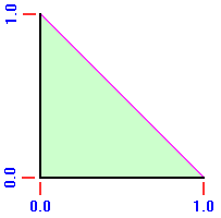
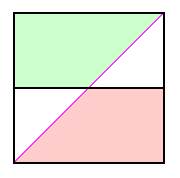
A graphical method elucidates how these considerations enter into the analysis. In Figure 1 the saddle and peak elevation correspond to the x and y-axes, respectively. Their scales are normalized such that 0 through 1 correspond to a single contour interval on the topographic chart. This includes both a shifting of each elevation, i.e. 12,000 feet becomes 0 feet; and a contraction of scale, i.e. a 40 foot contour interval becomes unit distance.
This normalization is performed so that every combination of contour interval and {peak, saddle} elevation pair can be displayed on a single graph. The resulting analysis then applies to all such combinations, be they realized in practice or not.
The given square region is part of a much larger set of squares which differ from it along the two dimensions of saddle and peak elevation. It is obvious that our analysis is complete by consideration of just this one square.
Importantly, a uniform distribution is assumed for mountain prominences, i.e. that within a narrow range of possible values, the probability of true prominence having a specific value is the same throughout that range. In the Appendix this assumption is dispensed with to demonstrate the effects of a more realistic prominence distribution.
The notation E (x) refers to the reported minus true saddle elevation, and similarly E (y) for the peak elevation. E (x, y) is the corresponding calculated minus true prominence, which when averaged over a sufficiently large sample of peaks yields the MSD (mean signed difference).
Case 1 - Peak and saddle elevations are both exactly known.
Reported and true prominence are identical in this case.
Case 2 - Peak elevation is exactly known; saddle elevation is unknown.
In Figure 1 the vertical line x = 0.5 corresponds to interpolated prominence's saddle elevation estimate. The y-coordinate, as peak elevation, is known. Hence the error in reported prominence is independent of y, and is given by E (x) = x - 0.5 where x is the true saddle elevation. By inspection E (x, y) results in an MSD of 0 and an MAE of 0.25, i.e. the mean absolute error of reported from true prominence is one-quarter a contour interval.
Case 3 - Neither the peak nor saddle elevation is known.
|
| Figure 2 |
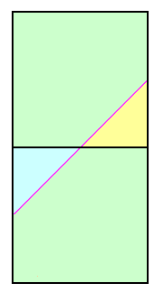
This is the only non-trivial case. Interpolated prominence estimates the (unknown) (x, y) by (0.5, 0.5). Thereby E (x, y) = (0.5 - y) - (0.5 - x) = x - y is the error in reported prominence. By inspection E (x, y) has an MSD of 0 since by symmetry the function x - y is zero when averaged over the entire square.
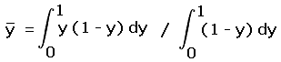
For calculating the MAE denote the reported prominence by Pinterp. Note that lines of slope 1.0 have constant prominence, ranging from a minimum of Pinterp - 1.0 at the lower right corner to Pinterp + 1.0 at the upper left corner. Referring again to Figure 1, by symmetry it is sufficient to consider just one-fourth of the square, chosen here as the triangle with right angle at the center (0.5, 0.5) and remaining angles at upper left and right.
In Figure 2 this triangle lies in the first quadrant with the side corresponding to Pinterp = 0.0 along the x-axis and the side extending (in Figure 1) from (0.5, 0.5) to (0.0, 1.0) along the y-axis. Its hypotenuse corresponds to the square's top in Figure 1.
Corresponding to the distance from Pmean = 0.0, and hence the unsigned deviation from
reported prominence, we must calculate the y-coordinate in Figure 2 as averaged over the entire triangle.
Denoting this value by  ,
,
 |
(1a) |
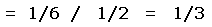 |
(1b) |
Hence the mean absolute error of reported from true prominence is one-third a contour interval.
Case 4 - Saddle elevation is exactly known; peak elevation is unknown.
This case is mathematically equivalent to Case 2 described above.
Thereby E (x, y) has the same distribution,
one with an MSD of 0 and an MAE of one-quarter a contour interval.
Case 1 - Peak and saddle elevations are both exactly known.
Reported and true prominence are identical in this case.
Case 2 - Peak elevation is exactly known; saddle elevation is unknown.
An analogous derivation applies as with Case 2 for interpolated prominence, except that the saddle elevation estimate, x = 0.5, is replaced by x = 1.0. From Figure 1 the mean signed difference, as the averaged of reported less true prominence, is by inspection -0.5. Hence on average clean prominence underestimates true prominence by one-half a contour interval.
The error distribution is uniform throughout the range 0.0 (when the true saddle elevation matches clean prominence's estimate) to -1.0 (when the true saddle elevation is at the contour's opposite end). Hence the mean absolute difference of clean prominence from its (nonzero) mean signed difference is by inspection one-quarter a contour interval.
Case 3 - Neither the peak nor saddle elevation is known.
Clean prominence estimates the (unknown) (x, y) by (1.0, 0.0), corresponding to the lower right corner of the square in Figure 1. For a given peak / saddle pair truly located at (x, y) the resulting error in reported prominence is (x - 1.0) - y, and is always negative-valued.
From symmetry arguments or by explicit integration of f (x, y) = (x - 1.0) - y over the unit square, one obtains a mean signed difference, as reported less true prominence, of -1.0, i.e. one full contour interval.
One obtains a mean absolute difference from the mean error of one-third a contour interval, having employed the same integration as with Case 3 of the interpolated prominence case.
Case 4 - Saddle elevation is exactly known; peak elevation is unknown.
This case is mathematically equivalent to Case 2 described above.
Thereby E (x, y) has the same distribution,
one with a mean signed difference of -0.5 and a mean absolute difference
from this (nonzero) mean signed difference of one-half a contour interval.
The same error distributions arise as with clean prominence, except that the sign is inverted,
i.e. all true prominences are overestimated.
This may be demonstrated with symmetry arguments and by direct calculation of each case.
Table 1 summarizes the error statistics for all three prominence definitions.
| Pinterp | Pmin | Pmax | |
| peak and saddle elevations known | 0.0 ± 0.0 | 0.0 ± 0.0 | 0.0 ± 0.0 |
| saddle OR peak elevation unknown | 0.0 ± 0.25 | -0.5 ± 0.25 | +0.5 ± 0.25 |
| peak and saddle elevation unknown | 0.0 ± 0.333 | -1.0 ± 0.333 | +1.0 ± 0.333 |
Table 1. Mean signed difference (MSD) and mean signed deviation of error
from MSD for various prominence definitions. The latter quantity is not
the mean absolute error (MAE). Values are in contour interval units.
Incorporation of Map Error and Refined Interpolation
From these results it is evident that only interpolated prominence merits further consideration. We now introduce map elevation error into the analysis, while also using refined peak and saddle elevation estimates based upon careful topographic chart scrutiny.
Map elevation error arises from both inaccurate map elevation contours and from inaccurate peak and saddle spot elevations. Then, error in calculated prominence derives from consideration of all elevations, be they contours and/or spot elevations, which contribute to its value.
Adjacent map elevation contour errors are assumed to be perfectly correlated, i.e. a 3 meter negative error in a saddle's lower bounding contour is accompanied by an identical negative error in the upper bounding contour. However map elevation contours that are distant from each other are assumed to have uncorrelated errors.
Spot elevation errors, being generally determined through a different method than nearby map elevation contours, are assumed to have errors which are uncorrelated with map elevation contour errors.
As with the previous subsection, we consider in-turn each permutation of known/unknown peak and saddle elevations, all the while recalling that only interpolated prominence is of interest. When spot elevations are not available the analysis applies equally well to refined interpolated prominence (RIP).
Case 1 - Peak and saddle elevations are both specified with spot elevations.8
This is the simplest case. We denote the standard deviation in spot elevation measurement by σ (elev). Assuming there is negligible systematic bias error, σ suffices to determine the RMS (root mean square) error in a large population of spot elevations.9 Conversely, given a published value for the RMS error, i.e. 3.3 meters, the standard deviation is immediately available.
Bias error is more critical for absolute heights than for prominences because biases due to systematic errors are similar for nearby locations (as peak and corresponding key saddle) and thus cancel.10,11
Assuming zero bias, prominence, as the difference of peak and saddle elevations, has a mean signed difference (MSD) of zero and a variance (squared standard deviation) of
| Var (p) = Var (peak) + Var (saddle) - 2 Cov (peak, saddle) (2) |
where Cov (peak, saddle) is the covariance of peak and saddle errors as averaged over a large population. Peaks of low magnitude prominence tend to have nearby saddles which might, depending on the measurement procedure, have similarly-signed elevation errors that result in a large magnitude covariance. From Equation 2 the resulting variance in prominence is expected to be small since the coviarance term nearly cancels the peak and saddle terms.
Peaks with large magnitude prominence tend to have distant saddles for which no such correlation in errors is expected. In that case the variance in calculated prominence, and hence standard error is simply the sum of peak and saddle variances.
In the British Ordnance Survey (OS) a maximum (3σ) error of ±3.3 meters is reported for spot elevations (and ±2 feet for trig points). Thus σ = 1.1 meters for both peak and saddle. Using Equation (2), and recalling that variance is the square of standard deviation, for distant peak-saddle pairs the prominence has a standard deviation of (2)1/2 x 1.1 meters = 1.56 meters (and 1 foot for a pair of trig points).
Case 2 - Peak elevation is specified with a spot elevation; saddle elevation is estimated using interpolation.
Equation (2) is applied. The covariance term is zero, recalling our assumption that peak spot elevations and map contour elevations have uncorrelated errors.
The peak elevation variance is the same as with Case 1 (1.21 meters2 in our example). Reference [12] reports an RMS error of 1.8 meters for 10 meter contours. Recalling that adjacent map elevation contour errors are assumed to be perfectly correlated, an interpolated saddle elevation has a variance as the sum of two contributions.
One contribution is the variance due to uncertainty in where between the upper and lower bounding contour elevations the saddle is located. For a uniform distribution this variance is one-twelfth the squared contour interval as shown by elementary integration - in our example 8.33 meters2.
The second contribution is 3.24 meters2 since the saddle's lower and upper bounding contours have synchronous elevation errors. Thereby the saddle elevation variance is 11.57 meters2. Adding to this value the peak elevation variance and taking the square root, we obtain a prominence standard deviation of 3.57 meters (and a meaned signed difference of zero). For a trig point-based peak elevation the corresponding value is 3.41 meters. Note how the majority of uncertainty in prominence stems from the saddle elevation's uncertainty.
Suppose that the saddle elevation is estimated using refined interpolation. Let the investigator decide that the saddle lies in the lowest one-third of the 10 meter contour interval. The calculation proceeds as above except that the squared contour interval is now one-ninth of its former value. Hence the variance due to uncertainty within the narrowed elevation range is 0.93 meter2. We add 3.24 meters2 due to uncertainty in the lower bounding countour's true elevation and the peak elevation variance of 1.21 meters2 to obtain a total variance of 5.38 meters2. Thus the prominence standard deviation is 2.32 meters - a significant reduction from 3.57 meters obtained by simply interpolating between bounding saddle contours. For a trig point-based peak elevation the corresponding value is 2.05 meters. Note how the trig point-based uncertainty in prominence is only slightly reduced from the spot elevation-based uncertainty.
Case 3 - Both peak and saddle elevations are estimated using interpolation.
Equation (2) is again applied. However the covariance term is nonzero for peak and saddle pairs in close proximity (such as occurs for mountains with small magnitude prominences). There are two limiting cases to be considered in the absence of an observation-based estimate for the covariance.
A. The covariance term completely cancels the peak and saddle variance terms.
This case may be approached for peak and saddle pairs in close physical proximity. However we must be careful: what gets canceled are only the variances due to inaccurate contour elevations. There remains variance owing to uncertainties in where, within their respective bounding contours, lie the true peak and saddle elevations.
Assuming the same 10 meter contour inverval, both peak and saddle contribute 8.33 meters2 to the variance. Hence the prominence standard deviation is 4.08 meters (and a meaned signed difference of zero). There is no special case for trig points since neither spot elevations nor trig point elevations are available in this case.
B. The covariance term is zero.
This case should occur for peak and saddle pairs which are distanced from each other, and as occurs for large magnitude prominences. For both peak and saddle adjacent bounding elevation contours rise and fall in-synchrony such that their respective variances are the sum of variance due to uncertainty in the mean contour elevation (3.24 meters2) and variance due to uncertainty of where within the bounding contour ranges they truly lie (8.33 meters2). The total variance is 23.15 meters2, such that the prominence standard deviation is 4.81 meters (and a meaned signed difference of zero). Again, there is no special case for trig points.
Case 4 - Saddle elevation is specified with a spot elevation; peak elevation is estimated using interpolation.
This uncommon case has the same prominence mean signed difference (zero) and standard deviation (2.32 meters)
as with Case 2.
For a trig point-based saddle elevation the latter value is 2.05 meters.
Table 2 summarizes the error statistics for all four cases above using examples specific to the British Ordnance Survey.
| prominence standard deviation | |
| peak and saddle elevations by trig point | ± 0.28 |
| peak OR saddle elevation by spot elevation the other one by trig point |
± 1.12 |
| peak and saddle elevations by spot elevation | ± 1.56 |
| Peak elevation by trig point; saddle elevation by contour interpolation (or vice-versa) |
± 3.41 |
| Peak elevation by spot elevation; saddle elevation by contour interpolation (or vice-versa) |
± 3.57 |
| nearby peak and saddle elevations estimated by contour interpolation |
± 4.08 |
| distant peak and saddle elevations estimated by contour interpolation |
± 4.81 |
Table 2. Standard deviation of calculated prominence for assorted permutations of elevation data availability.
In all cases the MSD (mean signed difference) is zero, having employed interpolated prominence.
Values are in meters.
8. "Trig points" are treated analogously, albeit with a different standard error. See Reference [9].
9. See this article on altitude corrections wherein an analogous derivation has been applied. 10. There is evidence for a +0.5m bias in saddle heights on British Ordnance Survey (OS) maps due to cols
Derivation of Gray Zone Peak List Assignment Probabilities
We demonstrate the effect of prominence definition choice on list candidacy status of "gray zone" peaks near the bottom of a prominence based peak list. The simpler case of neglecting map elevation contour errors (and errors in spot elevations) is considered. This is because nearly all of the key observations can be extracted from such analysis; and because the detailed calculations can be performed "analytically", i.e. without any numerical approximations. Map contour and spot elevation errors are subsequently included.
The same factors must be accounted for as when calculating prominence errors (as in the previous subsection).
In addition we have an extra consideration:
The reader is again referred to Figure 1.
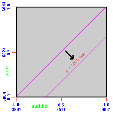
Let the prominence list have a 2,000 foot cutoff value, a most common figure in United States prominence lists. Then peaks of approximately 6,000 foot elevation are paired with roughly 4,000 foot key saddles as gray zone members. Furthermore let the contour interval be 40 feet as commonly present in USGS 1:24,000 scale topographic charts. Thus a measure of practicality is lent to this example. Then the point (1/2, 1/2) represents a peak and saddle pair with elevations of respectively 6,020 and 4,020 feet.
By inspection any pair lying on the diagonal y = x will have a prominence of exactly 2,000 feet. A pair lying below this diagonal has a prominence less than 2,000 feet; and a pair lying above this diagonal has a prominence exceeding 2,000 feet. The square contains peaks with prominences ranging from 1,960 feet (at the lower right) to 2,040 feet (at the upper left).
The (x, y) coordinates are true saddle and peak elevations - not our educated guesses of what they might be. Failure noting this point will result in confusion when following this subsection's text.
The given square region is part of a much larger set of squares which differ from it along the two dimensions of saddle and peak elevation. Squares located to the right lie completely in a region where all of the peaks lie below the cited diagonal and hence lack 2,000 feet of prominence. These squares need not be analyzed since, regardless of prominence type etc... the probability p of any corresponding peak having 2,000+ feet of prominence is 0.0.
Squares to the left are filled with peaks that are guaranteed to have at least 2,000 feet of prominence: p = 1.0. Squares above the square of Figure 1 contain peaks that, lying above the cited diagonal, also meet the list cutoff criterion. Finally squares below Figure 1 contain only peaks lacking 2,000 feet of prominence.
The only square that contains peaks for which it is uncertain of their 2,000 foot prominence status is that square displayed in Figure 1. Squares diagonally to its upper right and lower left are mathematically equivalent to the given square insofar as analyzing the desired peak list inclusion probabilities, as they represent (peak and saddle) pairs which differ in elevations by integer multiples of the specified contour interval, e.g. (3/2, 3/2) corresponds to a 6,060 foot peak with a 4,060 foot key saddle.
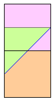
When Pcutoff is a half-integer multiple of the contour interval different statistics result. A pair of squares are analyzed as shown in Figure 3 wherein the specific, important case of Pcutoff = 300 feet is shown with a 40 foot contour interval.
The various combinations of prominence definition, knowledge of exact peak and/or saddle elevation and the ratio of Pcutoff to chart contour interval are considered.
Case 1 - Peak and saddle elevations are both exactly known.
The prominence is trivially available without any uncertainty in whether Pcutoff is met.
Thereby the probability of correctly identifying any peak as meeting this criterion is 1.0.
Case 2 - Peak elevation is exactly known; saddle elevation is unknown.
This is a nontrivial problem. With reference to Figure 1 we consider, for successive thoughtfully-selected true peak elevations, what is the probability that the resulting computed Pmean correctly places the peak on or off the prominence list.
|
| Figure 4 |
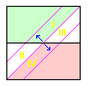
We begin with a 6,010 foot peak, corresponding (with a 40 foot contour interval) to the horizontal line y = 0.25. The mean saddle elevation is 4,020 feet. Hence the computed Pmean is 1,990 feet, insufficient for listing the peak. How often is that decision correct? It is that fraction of the line y = 0.25 to the lower right of the main diagonal, i.e. that triangle for which the true but unknowable prominence is less than 2,000 feet. By inspection that probability is 0.75.
Similarly, for a 6,000 foot peak that probability is 1.0 as the entire line is 0.0 lies below the diagonal. Similarly, for a 6,020 foot peak we have 0.5 as the probability. The totality of cases for peaks between 6,000 and 6,020 feet inclusive wherein they are correctly left off the list is represented at right in Figure 4 by the light pink-colored region.
A completely analogous analysis is applied for peaks between 6,020 and 6,040 feet, inclusive, except that now we wish the peaks to be (correctly) assigned on the final list. The totality of cases for these peaks 6,000 and 6,020 feet inclusive wherein they are correctly left off the list is represented in Figure 4 by the light green-colored region.
|
| Figure 5 |
The pink and green regions collectively occupy three-fourths of the square in Figure 4. Thereby the averaged probability of correctly identifying peaks as meeting the list cutoff criterion is 0.75.
The above derivation pertains to when Pcutoff is a multiple of the contour interval. When Pcutoff is a half-integer multiple of the contour interval different statistics result. A pair of squares are required as shown in Figure 3 wherein the specific, important case of Pcutoff = 300 feet is shown with a 40 foot contour interval.
The calculated prominence is (known) peak elevation minus the mean saddle elevation of 620 feet. Within the upper square the minimum peak elevation is 920 feet. Hence the entire square's peak set is considered listworthy. The true prominence is at least 300 feet for all points except the light yellow-colored triangle of Figure 5. Thus for this square Pinterp correctly predicts list membership 7/8 of the time (all but the yellow region).
Within the lower square the calculated difference is never at least 300 feet since here the maximum peak elevation is 920 feet. Hence no peaks are considered to have met the prominence cutoff value, a notion which is correct 7/8 of the time (all but the blue colored triangle in Figure 5).
Taken collectively, mean prominence has correctly placed peaks on (or off) the prominence list 7/8 of the time (0.875).
Case 3 - Neither the peak nor saddle elevation is known.
Two cases arise in practice depending on whether Pcutoff is a multiple of the contour interval
or a half-integer multiple thereof. We consider each case in-turn.
A. Pcutoff is a multiple of the contour interval. The current example suffices as 2,000 feet
is a multiple of 40 feet. The mean peak elevation is 6,020 feet and the mean saddle elevation is 4,020 feet.
Hence the computed prominence is 2,000 feet regardless of where the (peak, saddle) point is in-truth located
within the square. This meets the 2,000 foot cutoff criterion every time. However the true peak and saddle elevations
lie above the main diagonal just one-half the time.
Thereby the averaged probability of correctly identifying peaks as meeting the list cutoff criterion is 0.5.
|
|
| Figure 5 |
B. Pcutoff is a half-integer multiple of the contour interval. The most prevalent example is when Pcutoff = 300 feet and we have a 40 foot contour interval (300 / 40 = 7.5). Thus our square could represent peaks from 920 to 960 feet with key saddles from 600 to 640 feet. The mean peak elevation is 940 feet and the mean saddle elevation is 620 feet for a computed prominence of 320 feet. Thus all (peak, saddle) pairs meet the 300 foot cutoff value and are placed on the prominence list.
How often is that decision correct? It is simply that fraction of the square's area occupied by (peak, saddle) pairs for which the true prominence is at least 300 feet. By inspection this occurs throughout the upper square of Figure 5 except for the small light yellow triangle at the square's lower right. That triangle occupies one-eighth of the square.
Now let our square represent peaks from 880 to 920 feet with key saddles as previously. The mean peak elevation is 900 feet and the mean saddle elevation is 620 feet for a computed prominence of 280 feet. Thus all (peak, saddle) pairs fail the 300 foot cutoff value and are left off the prominence list.
How often is that decision correct? It is simply that fraction of the square's area occupied by (peak, saddle) pairs for which the true prominence is less than 300 feet. By inspection this occurs throughout the square except for the small triangle at the square's upper left shown by light blue in Figure 5. That triangle occupies one-eighth of the square.
We conclude that the averaged probability of correctly identifying peaks as meeting the list cutoff criterion is 0.875 (seven-eighths).
Case 4 - Saddle elevation is exactly known; peak elevation is unknown.
This unusual case has already been solved upon noting that the square knows nothing of mountains - it is a mathematical tool only. One may denote the (real) saddle as "peak", the (real) peak as "saddle", and compute the resulting pair's "negative prominence". Using the results of Case 2 we obtain the averaged probability of correctly identifying peaks as meeting the list cutoff criterion as 0.75 for the integral multiple result, and 0.875 for the half-integral multiple value.
Table 3 reviews these various cases for an interpolated prominence definition.
| Pcutoff contour interval integer multiple |
Pcutoff contour interval half-integer multiple |
|
| peak and saddle elevations known | 1.0 | 1.0 |
| saddle OR peak elevation unknown | 0.75 | 0.875 |
| peak and saddle elevation unknown | 0.5 | 0.875 |
Table 3. Probabilities of correctly identifying gray zone peaks as meeting a list cutoff using interpolated prominence.
Contour elevation and/or spot elevation error is not included.
Case 1 - Peak and saddle elevations are both exactly known.
As in the interpolated prominence case, the prominence is trivially available without any uncertainty in whether
Pcutoff is met.
Thereby the probability of correctly identifying any peak as meeting this criterion is, again, 1.0.
Case 2 - Peak elevation is exactly known; saddle elevation is unknown.
As with mean prominence there are two possible statistics depending on whether Pcutoff is an integral multiple or a half-integer multiple of the contour interval.
A. Pcutoff is a multiple of the contour interval.
The case of Pcutoff = 2,000 feet is used again, as are peaks of approximately 6,000 foot elevation paired with 4,000 foot key saddles. The contour interval remains 40 feet. Prominence is computed using the maximum possible saddle elevation of 4,040 feet. Hence prominence is peak elevation minus 4,040 feet. However the peak elevation is always less than 6,040 feet. Hence the calculated prominence is always less than the 2,000 foot cutoff value for list inclusion. The diagonal line of Figure 1 separates peaks which truly have at least 2,000 feet of prominence, to its upper left, from peaks which do not meet this cutoff value to the lower right. Thereby the averaged probability of correctly identifying peaks as failing the list cutoff criterion is 0.5.
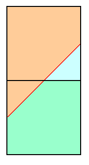
B. Pcutoff is a half-integer multiple of the contour interval.
|
| Figure 6 |
We refer again to Figure 3 wherein the specific, important case of Pcutoff = 300 feet is shown with a 40 foot contour interval.
The calculated prominence is (known) peak elevation minus the maximum saddle elevation of 640 feet. Within the upper square this difference is at least 300 feet for it's top one-half, a region where the true prominence is indeed at least 300 feet. Within the upper square this difference is less than 300 feet only for the small triangle at its lower right; and, for this triangle, the true prominence is indeed less than 300 feet. The triangle has an area of 1/8 the upper square. Hence in that region clean prominence correctly assigns peaks 5/8 of the time. Figure 6 shows these areas of correct peak assignment in light violet.
Within the lower square this difference is never at least 300 feet since its maximum peak elevation, 920 feet, yields a calculated 280 foot prominence. Within this square the true prominence exceeds 300 feet only for the small triangle at its upper left with 1/8 the square's area. Hence in the lower square clean prominence correctly assigns peaks as not on the list 7/8 of the time (light orange in Figure 6). Noting the upper and lower square's respective correct prediction rates, the averaged probability of correctly identifying peaks as meeting the list cutoff criterion is 0.75 (three-fourths).
Case 3 - Neither the peak nor saddle elevation is known.
A. Pcutoff is a multiple of the contour interval.
Here calculated prominence is given by the minimum possible peak elevation less the maximum possible saddle elevation. For the same Pcutoff = 2,000 feet example this is 6,000 feet - 4,040 feet = 1,960 feet. Hence clean prominence denies every peak from list inclusion. This is correct only for peaks below and right of the diagonal in Figure 1. Hence clean prominence correctly assigns peaks 1/2 of the time.
|
| Figure 7 |
B. Pcutoff is a half-integer multiple of the contour interval.
For the upper square of Figure 3 the calculated prominence is maximum saddle elevation minus minimum peak elevation = 920 feet - 640 feet = 280 feet. Hence clean prominence denies every peak from list inclusion (as Pcutoff = 300 feet). The true prominence is under 300 feet only 1/8 of the time, specifically, in the upper square's lower right triangle (light blue in Figure 7).
For the lower square of Figure 3 the calculated prominence is 880 feet - 640 feet = 240 feet. Again, clean prominence denies every peak from list inclusion. The true prominence is under 300 feet fully 7/8 of the time, specifically, everywhere except the lower square's upper left triangle and shown as light green in Figure 7. Noting the upper and lower square's respective correct prediction rates, the averaged probability of correctly identifying peaks as meeting the list cutoff criterion is 0.5.
Case 4 - Saddle elevation is exactly known; peak elevation is unknown. As shown, this case is mathematically equivalent to Case 2 described above. Thereby the same statistics result.
Table 4 reviews these various cases for a clean prominence definition.
| Pcutoff contour interval integer multiple |
Pcutoff contour interval half-integer multiple |
|
| peak and saddle elevations known | 1.0 | 1.0 |
| saddle OR peak elevation unknown | 0.5 | 0.75 |
| peak and saddle elevation unknown | 0.5 | 0.5 |
Table 4. Probabilities of correctly identifying gray zone peaks as meeting a list cutoff using
clean and optimistic prominence.
Contour elevation and/or spot elevation error is not included.
The same probabilities of correct gray zone peak placement arise as with clean prominence.
This may be demonstrated with symmetry arguments and by direct calculation of each case.
Hence Table 4 applies equally well to optimistic prominence.
Incorporation of Map Error into Gray Zone Peak List Assignment
General Considerations
|
| Figure 8 |
Map contour errors enter by shifting the position of squares relative to the diagonal line corresponding to Pcutoff . Figure 8 is identical to Figure 1 apart from a 9 foot map overestimate of bounding saddle contours and a 4 foot underestimate of bounding peak contours.
Figure 8 coordinates are true elevations. Hence a true 3,991 foot bounding saddle contour elevation is erroneously concluded to be 4,000 feet. Similarly a true 4,044 foot bounding peak contour elevation is erroneously concluded to be 4,040 feet. Lower and upper bounding saddle contours have identical elevation errors because they are measured simultaneously. Hence the same measurement bias results - and similarly for the pair of bounding peak contours.
The net result of these contour elevation errors is to shift the diagonal line corresponding to Pcutoff by 9 + 4 = 13 feet.
Let the prominence be estimated by interpolation. Furthermore let Pcutoff be an integer multiple of the contour interval, and as satisified with the (2000 foot, 40 foot) pair of Figure 8. From previous arguments the probability of correct peak placement is 0.5 when the diagonal line representing Pcutoff has not been shifted. When the diagonal is shifted to the lower right more than one-half of peaks have in-truth at least 2,000 feet of prominence since the corresponding fraction is simply that portion of the square to the diagonal's upper left.
However our current +13 foot shift in mean prominence for the entire square's set of peaks could just as readily have been a -13 foot shift, and as caused by net underestimate in the four bounding contour elevations. There by we conclude that, after averaging over the entire population of peaks and their corresponding saddles the net (unsigned) shift in placement of the diagonal line representing Pcutoff is zero.
The analysis differs for when spot elevations for both peak and saddle are available. For suppose that in Figure 1 we select a point (x, y) corresponding to a specific peak and key saddle pair for which spot elevations are provided. An error circle exists around that point corresponding to the spot elevation errors. We are no longer certain if the true (x, y) coordinates lie on the same side of the Pcutoff diagonal as do the measured pair of coordinates. Hence there is a finite yet small chance that the calculated prominence will incorrectly miscategorize the peak insofar as inclusion on the prominence list.
The final case is considered wherein we retain the (2000 foot, 40 foot) pair and provide just the peak with a spot elevation, i.e. for the saddle we have only the bounding contour elevations to work with. From the previous analysis for interpolated prominence the probability of correct peak list assignment is 0.75.
|
| Figure 9 |
Figure 9 illustrates the situation, being identical to Figure 4 apart from including net shifts in the diagonal line corresponding to Pcutoff. Those net shifts arise from an error ellipse centered at any given peak and saddle coordinate pair corresponding to the (generally larger magnitude) uncertainty in saddle elevation (due to bounding contour elevation error), and the (generally smaller magnitude) uncertainty in peak elevation (due to spot elevation error).
A net shift to the upper left raises the small, white triangle's area on the right side corresponding to incorrectly assigning peaks to the list (region I); while lowering the small, white triangle's area on the left side corresponding to erroneously not listing peaks (region II). The increase in one triangle's area exceeds the decrease in the other triangle's area (area of I > area of II). There is a net increase in the probability of incorrect peak list assignment.
A net shift to the lower right lowers the small, white triangle's area on the right side corresponding to incorrectly assigning peaks to the list (region III); while raising the small, white triangle's area on the left side corresponding to erroneously not listing peaks (region IV). The increase in one triangle's area exceeds the decrease in the other triangle's area (area of IV > area of III) There is again a net rise in the probability of incorrect peak list assignment.
By symmetry arguments the same conclusion is reached upon reversing our state of knowledge, i.e. the saddle has a spot elevation while the peak does not.
13. Careful analysis of adjacent squares reveals that for clean and optimistic prominence there is a net increase in the error rate.
Quantitative Probabilities with Inclusion of Map Errors
It is reasonable to assume that map elevation errors are described by normal distributions, referred to colloquially as the "bell curve". The algebraic expression of this curve does not permit exact, so-called analytic evaluation of the desired probabilities. Numerical methods are thus required.
One applies such a prescription to quantitatively address any of several problems. We limit considerations to that subset of gray zone peak assignment issues, wherein the inclusion of map elevation errors arises in zeroth order, i.e. provides the main contribution to final calculated peak misassignment rates. This occurs when the misassignment rate is predicted to be zero in the absence of explicit map elevation error consideration.
The following list of interesting calculations results.
|
| Figure 10 |
We emphasize that these specific problems are considered because for each one, map elevation errors transform a zero probability of peak miscategorization into a finite yet small probability. In contrast, other interesting problems related to map elevation errors merely raise by a fraction the peak miscategorization probability relative to ignoring their effects.
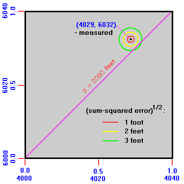
Consider PROBLEM A with Figure 10 as reference. A peak of measured elevation 6,032 feet has a key saddle of measured elevation 4,029 feet. By any prominence definition the prominence is 2,003 feet. Centered about that peak (represented by a black dot) are concentric circles of increasing radii corresponding to unit foot increments in the square root of the summed squares of the peak and saddle measurement errors in feet. Thus the yellow circle contains the true (saddle, peak) point if the peak elevation error is ±2 feet and the saddle measurement is spot-on, and similarly for other combinations of saddle and peak measurement errors so long as their summed square is 4 feet2.
The green circle demonstrates how a sufficiently large composite error in measured elevations can place the true (saddle, peak) point below the main diagonal corresponding to the prominence list cutoff value. In the present case we require some combination of saddle and peak errors sufficiently large in magnitude, and of the appropriate signs, to place the true (saddle, peak) point below the main diagonal.
Our task is computing the probability of this event as a function of the perpendicular distance of the measured point to the main diagonal given known standard errors for the two elevation measurements. This perpendicular distance is by inspection the calculated prominence minus Pcutoff , and is simply y - x.
Let the true (saddle, peak) pair have coordinates (xo, yo). Then the saddle measurement error, x - xo, is normally-distributed with a mean of 0 and a standard deviation σ (elev) determined by the measurement methodology. The peak measurement error y - yo is normally-distributed similarly. Importantly, there is no reason to suspect a measurement bias, one which would in any event simply shift the distribution's mean while leaving the all-important variance uneffected. We shall also assume there is no correlation between peak and saddle measurement errors.
Under these approximations we have a combination of two independent
standard normal random variables as
{(x - xo)/σ (elev), (y - yo)/σ (elev)}.
Thereby we apply the
following result:
PROBLEM A is reduced to evaluating the probability that a standard normal random variable has a value equal to at least |calculated prominence - prominence cutoff | / [21/2 σ (elev)], where the absolute value signs allow for the case of Pcalc < Pcutoff.
The required cumulative distribution function (CDF) of the normal distribution cannot be written in closed form. However detailed tabulations and numerical approximations are available. Thereby in Table 5a benchmark values are provided for various ratios of |Pcalc - Pcutoff | / σ (elev). Here Pcalc is any prominence definition type and the 21/2 factor is implicitly accounted for in the tabulated results.
| |Pcalc - Pcutoff | / σ (elev) | peak misassignment probability |
| 0.0 | 0.50 (50%) |
| 1.0 | 0.2398 (24%) |
| 2.0 | 0.0787 (7.9%) |
| 3.0 | 0.0170 (1.7%) |
| 4.0 | 0.0023 (0.23%) |
| 5.0 | 0.0002 (0.02%) |
Table 5a. Problem A. Probability of misassigning a gray zone peak as a function of
the difference between reported prominence and the list cutoff value
when both peak and saddle elevations are measured.
Let the spot elevation measurements have a standard error of σ (elev) = 3 feet. Then for a peak with calculated prominence of 1,994 feet we have |Pcalc - Pcutoff | / σ (elev) = 2.0. From Table 5a the probability this peak is erroneously left-off a 2,000 foot prominence list is 7.9%. Similarly let another peak have a 2,003 foot calculated prominence. Now the probability of mistakenly having listed this peak is 24% - about one chance in four, requiring only that the combined saddle and peak measurements have overestimated by at least 3 feet.
Finally, by symmetry a peak with exactly 2,000 feet calculated prominence has a 50% chance of being incorrectly placed. However the probability of a measured (saddle, peak) pair lying exactly on the main diagonal is infinitesimal (after disregarding round-off error considerations).
This formalism is next applied to answer a second question of wide applicability -
We thereby replace the notion of "saddle" with "peak X elevation" and of "peak" with "peak Y elevation". The peak X measured elevation error X (error) is x - xo, and for peak Y we have Y (error) = y - yo. Each of these differences is normally-distributed with a mean of 0 and with standard deviation σ (elev). Hence their difference, as Y (error) - X (error), is also a normal random variable, one with variance 2 σ (elev). Substituting, Y (error) - X (error) = (y - yo) - (x - xo) = (xo - yo) + (y - x).
The true peak X elevation minus the the true peak Y elevation is xo - yo. How often is this value positive such that the true elevation of peak X exceeds that of Y? Substitution into the expression for Y (error) - X (error) of xo - yo > 0 shows this occurs when Y (error) - X (error) > (y - x). Now y - x is simply the difference in the peak's measured elevations. Hence peak X is higher than peak Y when the normal random variable Y (error) - X (error) exceeds the two peak's measured elevation difference.
Table 5b provides the required minimum measured elevation difference for peak Y to truly be higher than peak X at difference levels of confidence. The table's numerical values are useful for PROBLEM A as well.
| confidence | (peak Y (measured) - peak X (measured)) / σ (elev) |
| 50% | 0.0 |
| 75% | 0.954 |
| 90% | 1.812 |
| 95% | 2.326 |
| 99% | 3.290 |
| 99.9% | 4.370 |
Table 5b. Required measured elevation differences for peak Y being truly higher than peak X,
the difference normalized by measurement standard error σ (elev),
at different confidence levels.
Consider a actual example taken from Colorado's San Juan Range. Here, Windom Peak and Mount Eolus compete for the title of La Plata County highpoint. Their benchmark elevations are respectively 14,082 and 14,083 feet. Dave Covill reports that the Eolus summit benchmark is about one foot below the highest ground; while the Windom benchmark is fully 4 feet 6 inches below the highest rock. Thus the measured summit elevations are 14,086.5 feet and 14,084 feet for Windom Peak and Mount Eolus, respectively.
From Table 5b one may be 90+% confident provided that the standard benchmark measurement error is no greater than 2.5 feet / 1.812 = 1.38 feet. The corresponding figures for 75+% and 99+% confidence are respectively 2.62 feet and 0.76 feet. The latter high accuracy is unlikely to be satisfied.
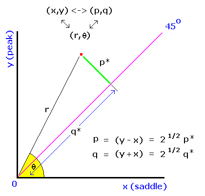
The peak and saddle elevations define a coordinate pair (x, y) in the plane's first quadrant.14 Consider a transformation of variables from (x, y) to (p*, q*) where
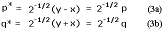 |
In Eqs.(3a,b) p is the familiar topographic prominence. q is the orthogonal coordinate specifying the exact placement of a point along any diagonal line of constant p. These equations define a 45 degree rotation in (peak, saddle) space, wherein the x and y-coordinates (saddle and peak elevations) are transformed to q and p, respectively.
|
| Figure 11 |
q is prominence's antithesis, in a sense, being maximized for mountains with high peak and saddle elevations. To see this, subtract Equation (3a) from Equation (3b) to obtain q - p = 2x, i.e. a high saddle elevation, x, corresponds to large magnitude q yet small magnitude p.
Figure 11 illustrates the relationships herein described.
(Peak, saddle) pairs above sea level lie in the first quadrant
between 45 and 90 degrees (as peak elevation must be at least saddle elevation, such that y ≥ x).
From Eqs.(2a,b) we have p = r (sin  - cos )
and q = r (sin + cos )
where (r, ) are the plane polar coordinates of a (peak, sadde) pair.
- cos )
and q = r (sin + cos )
where (r, ) are the plane polar coordinates of a (peak, sadde) pair.
Within this 45 degree-wide slice sin - cos
is minimal at 45° with a 0 value. Hence prominence is 0 as at 45° the saddle and peak elevations are equal.
Prominence increases with for a fixed value of r.
Similarly sin + cos is maximal at 45°.
Hence q increases (albeit at a slow rate) as the line of zero prominence is approached for a fixed value of r.
A connection with orometrical dominance is made. Defined as prominence divided by peak elevation,
we have dominance d = p/y = (y - x)/y = 1 - x/y = 1 - cot .
Hence dominance assumes its maximal value of 1.0 along the y-axis
(where is 90°), and diminishes to its minimal value of 0.0
when = 45°.
This angular-dependence is reminiscent of how p varies with ,
and as demonstrated algebraically in terms of the orthogonal pair (p,q): d = p/y = 2p/(p+q).
Hence large q correlates with small dominance.
Just as dominance is largest for island and continental highpoints (because the saddle lies at sea level), so too q prefers continent-bound subpeaks of high elevation and little prominence. "Prominent" examples include the south peak of Mount Everest, Denali's North Peak and whichever summit at Ojos del Salado is the lower of two candidates.15
Finally recall that q is defined as that coordinate at right-angles to prominence at any point in (peak, saddle) space. Its value changes when prominence is fixed, and it is fixed in value when prominence changes. Given this attribute and the above description we are tempted to conclude that
14. (Peak, saddle) pairs lying below sea level will lie elsewhere. However it's impossible for
any pair to lie in the half-plane from 0 to 45° and from 225 to 360°
as that requires a key saddle elevation exceeding the corresponding peak elevation.
We again begin with the simpler case of neglecting map errors, incorporating them later. From Table 1 the mean signed difference (MSD), as calculated prominence less true prominence, is zero for interpolated prominence and one-half a contour interval for other definitions when only the peak or only the saddle elevation is known with precision. The error's sign is negative for Pmin and positive for Pmax.
When neither the peak nor saddle elevation is precisely known these latter mean signed differences double to a full contour interval. Meanwhile Pinterp still provides a zero MSD.
Although Pmin and Pmax are biased estimators of the true prominence, the simple prescriptions
 |
(4a) |
and
 |
(4b) |
recover the same zero mean signed difference enjoyed by Pinterp.
In Eqs.(4a,b)  is the topographic chart contour spacing.
f = 0.5 for the case of known peak (or saddle) elevation, and similarly
f = 1.0 for when both elevations are uncertain.
is the topographic chart contour spacing.
f = 0.5 for the case of known peak (or saddle) elevation, and similarly
f = 1.0 for when both elevations are uncertain.
From Table 1 the mean absolute error (MAE) is independent of prominence definition, and is a function only of whether the peak (or saddle) elevation is precisely given. When exactly one of the latter values is provided the mean absolute error (as measured from the MSD) is one-fourth the contour interval, e.g. 10 feet with a 40 foot chart. When neither the peak nor saddle elevation is precisely known the mean absolute error (again, measured from the MSD) rises to one-third the contour spacing - 13 feet 4 inches with a 40 foot map.
In the remaining subsections devoted to error analysis only interpolated prominence is considered.
Effects of Inaccuracies in Published Chart Elevations
Several important points derive from the results of Table 2. Contributions to prominence standard deviation
arise from three general sources.
In descending order of magnitude,
Indeed, because a square root is taken to obtain prominence standard deviation ("PSD"), the additional PSD caused by contour and spot elevation errors relative to existing uncertainty in location of saddle (or peak) within a bounding contour pair (and error due to contour elevation error) is fractionally small. Geometrically this corresponds to the hypotenuse of a sharp-angled right triangle being minimally larger than the acute angle's near side.
The fourth and fifth entries of Table 2 illustrate this point. We include a phantom entry corresponding to "peak elevation has no error, spot elevation by contour interpolation (or vice-versa)". The resulting PSD of ±3.40 meters is marginally smaller than the tabulated values of ±3.57 meters and ±3.41 meters.
Further, the additional PSD caused by ALL errors apart from existing uncertainty in location of saddle (or peak) within a bounding contour pair is fractionally small. Again using the fourth and fifth entries for comparison, an entry corresponding to just inclusion of uncertainty in location of saddle (or peak) within a bounding contour pair has a PSD of ±2.89 meters (as the square root of 8.33 meters2), i.e. all but 19% and 15% of the PSD values for entries 4 and 5, respectively.
This is the justification for a two-step prominence error analysis, wherein map errors are considered secondary. One may conceive of the variance in calculated (interpolated) prominence due to location of saddle (and/or peak) within a bounding contour pair (or pairs) as a zeroth-order approximation to the final, calculated value. Incorporation of contour and spot elevation errors arise as correction terms.
The above conclusions require modification for United States contour elevation spacings and map errors. A typical contour spacing is 40 feet. Hence the variance in PSD due to uncertainty in location of saddle (or peak) within a bounding contour pair is 133.3 feet2 (as one-twelfth of 40 squared). The USGS claims that 90% of features lie within one-half a contour interval of their true elevations. For a normal distribution 90% of the area lies within ±1.645 standard deviations of the mean. Hence we obtain σ = 20 feet / 1.645 = 12.16 feet.
If we allow contour elevations to fall under this generic "feature" category, then uncertainty in bounding contour elevation contributes to PSD a variance equal to σ squared : 147.8 feet2. Hence in the USA contour elevation error contributes in roughly equal measure to PSD as does uncertainty in location of saddle (or peak) within a bounding contour pair.
Spot elevations would be of little merit if they were similarly crude estimates of true elevation. Hence we assume that they are more accurate and thus contribute in minor fashion to PSD - just as they do in the United Kingdom.
The USA σ of 3.71 meters for contour elevation error compares most unfavorably to the UK σ of 1.8 meters. However upon normalization by their respective total ranges of elevation a much more even-handed result obtains because Mount Whitney is over three times the height of Ben Nevis.16
16. Alaska's Denali is not included because Alaskan topographic charts have different contour spacings than for the remaining USA.
Refining Estimated Peak and Saddle Elevations
Sometimes one may narrow the range of a peak or saddle elevation by careful scrutiny of the corresponding topographic chart. Ultimately this yields a more accurate calculated prominence since its standard deviation, PSD, is diminished relative to what it is based solely on the map's contour interval and inherent errors.
This practice of "refined interpolated prominence" (RIP) is seldom employed in the United States. However prominence-oriented climber Rob Woodall of the United Kingdom has the following comments.
"In the UK we always estimate summit and/or saddle elevations (in the absence of spot heights or where the spots heights appear not to be at the summit/saddle) by visually interpolating between contours to the nearest metre.
I'm not aware that interpolated prominence in the sense used in the USA has ever been used in the UK. Only one early list I can think of (Corbetts) required a minimum number of contour rings, i.e. clean prominence."
Similarly, for Norway the following account is provided by Petter Bjørstad. Certainly examples can be found from other regions, each with peculiar land features that might enable improved elevation estimates.
"I interpolate between contours for all lists of my concern. Topo-maps in Norway have a 20 meter contour interval, but there are higher accuracy maps that cover populated areas, including most roads etc.... These maps have 5 meter contours, sometimes they even extend up to peaks. Most peaks have very accurate spot elevations, almost always to 1 meter, often down to one centimeter (laser-based surveys). Saddles are less well documented and thus need interpolation.
When doing this, there is one fact that seems natural adding into the calculation: We have thousands of small and larger lakes. Lakes nearly always have a spot elevation on them (or a range, say 943-978 meters, if the lake is part of a hydroelectric power system). By examining a lake with known elevation near a saddle, one may often reduce the interval of uncertainty (typically 20 meter), to a much smaller interval, often only 3-7 meter. This refined interval can then be interpolated.
Terrain is normally rugged and unpredictable, so estimates made on the basis of distance between contours etc... are generally unreliable. However, if one makes a visual, on-site inspection of the saddle, then an estimate based on the map combined with what the land looks like (saddles are often very flat wet meadows), then some improvements may be possible."
Note how neither clean nor optimistic prominence are capable of refinement in this fashion. These measures are poor starting points for narrowing the ranges of calculated prominences because they are biased estimators for the true prominence, i.e. their mean signed differences (MSD) are not zero.
The author is concerned that RIP might have a purely subjective component when the map reader judges
a saddle to lie in a narrow elevation range based solely on distances to adjacent map contours.
In contrast, if a nearby lake spot elevation serves to delimit a saddle's range of possible elevations
there is no such subjectivity.
Gray Zone Peak List Assignment Probabilities
From Tables 3 and 4 interpolated prominence correctly assigns list membership to gray zone peaks more reliably than does clean and optimistic prominence.
This observation is not qualitatively altered upon consideration of map contour and spot elevation errors as seen by the arguments of this subsection. Hence there is no discussion of their incorporation into the formalism except for the surprising result that a peak's clean prominence at least equal to the list cutoff value does not guarantee that it truly satisfies that cutoff criterion.
The extent of this reliability difference resides with two factors - whether the peak elevation is known
and whether Pcutoff is an integer or half-integer multiple of the contour interval.
When both the saddle and peak elevations are unknown and Pcutoff is an integer multiple of the contour spacing, interpolated prominence has no advantage in this matter: all definitions mis-assign peaks fully one-half the time.
However for large prominence peaks the elevation generally is known, whence interpolated prominence is a more reliable predictor of list status for gray zone peaks. Specifically, for lists with Pcutoff an integer multiple of the contour interval, interpolated prominence assigns peaks correctly three-fourths of the time while clean and optimistic prominence correctly assign peaks one-half the time. A common example is Pcutoff = 2,000 feet with a 40 foot contour spacing.
For small prominence peaks the elevation is generally unknown. The most important example is when Pcutoff = 300 feet with a 40 foot map contour spacing. Hence Pcutoff is a half-integer multiple of the contour spacing. With this combination of peak elevation uncertainty and Pcutoff to contour spacing ratio, interpolated prominence correctly assigns peaks seven-eighths of the time. Clean and optimistic prominence correctly assign peaks one-half the time.
This is a significant advantage for interpolated prominence - a statistic worthy of note for anybody interested in 300 foot prominence lists since a sizeable fraction of them will indeed be comprised of gray zone peaks.
Consider how to leverage the reliability of interpolated prominence for gray zone peak list assignment. From Tables 3 and 4 any prominence definition unambiguously assigns peaks when both peak and saddle elevations are known. Hence there is no preference for one prominence definition based on this criterion. Apart from this obvious result, and regardless of whether the peak elevation is known, interpolated prominence correctly assigns gray zone peaks with an impressive P = 0.875 - seven-eighths of the time when Pcutoff is a half-integer multiple of the map contour spacing.
Thus if a metric map's small prominence summits are to be documented, consider the use of a 90 meter Pcutoff when the contour interval is 20 meters since 90/20 is 4.5 - a half-integer. This is a common map spacing for Mexican topographic charts and elsewhere in Latin America. Furthermore, 90 meters is very close to 300 feet (it is 295.276 feet).
International peakbaggers generally use Pcutoff = 600 meters as a close analogue of the commonly employed 2,000 foot Pcutoff in the United States. Somewhat unfortunately, 600 is an even multiple of many possible metric map contour intervals - including 5, 6, 10, 12, 15, 20, 24, 25, 30, 40, 50 and 60 meters! Choose the interval and it's likely that interpolated prominence will therefore correctly assign gray zone peaks 3/4 of the time when the peak elevation is known - and only 1/2 of the time when it is not known.
However use of Pcutoff = 610 meters provides the desired half-integer multiple of a 20 meter contour interval. Furthermore at 2,001.312 feet, this cutoff value very closely aligns with the USA 2,000 foot Pcutoff value.
Conversely, were American lists to employ Pcutoff = 1,980 feet instead of 2,000 feet, the corresponding lists would correctly assign gray zone peaks occurs fully 7/8 of the time. Furthermore, peaks hitherto considered only to have at least P2000 feet of optimistic prominence would suddenly be listed.
The 5,000 foot cutoff value of ultra prominence peak lists is an even multiple of 40 feet but a half-integer multiple of 80 feet. Hence 80 foot maps, the less precise, ironically provide a larger probability of correct gray zone peak assignment! The international standard of Pcutoff = 1,500 meters is an even multiple of many possible metric map contour spacings including 10, 15 and 20 meters. It is a half-integer multiple of 40 meters (1500 / 40 = 37.5), such that, again, the less precise map results in a larger fraction of correctly assigned gray zone peaks.
There are always more small prominence than large prominence peaks for any geographic region or mountain range.
Together with the relatively large ratio of contour spacing / Pcutoff for a P300 foot list,
the fraction of peaks in its gray zone is considerably larger than for, say, a P2000 foot list - and even more so than for
an ultra prominence peak list. Hence the desirability of a half-integer multiple criterion for Pcutoff
is greatest for small prominence lists as this criterion only effects the performance of prominence definitions
in correct list assignment for gray zone peaks. Hence is it a fortunate "coincidence" that Pcutoff
of 300 feet has been chosen for general use at the small prominence regime, while leaving integer-multiple
Pcutoff values for medium and large prominence peak lists.
Effects of Nonuniform Prominence Distribution
Shift in Probabilities for Gray Zone Peak List Assignment
The statistics of Tables 3 and 4 assume that every point (x, y) of
Figures 1 and
3
are equally likely to be realized in practice.
In so doing probabilities are extracted simply as area ratios. This is not strictly true as
low prominence peaks are more frequent. As prominence is given by y - x,
in the Appendix
a more exact treatment is provided wherein the probability density
 (x, y) is an explicit
function of independent variable p = y - x.
(x, y) is an explicit
function of independent variable p = y - x.
Whereas familiarity with the Appendix is optional, the following considerations are central to this discussion. It is known that prominence density (the number of peaks per unit prominence per unit area) scales roughly according to a Power Law,
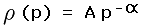 |
(5) |
where  is a small magnitude, positive exponent that varies by region.
Although the choice = 2.0 is
theoretically suggested, empirically the author has found that for small prominences
(i.e. at the bottom of a P300 foot list) a better choice is = 1.5.
is a small magnitude, positive exponent that varies by region.
Although the choice = 2.0 is
theoretically suggested, empirically the author has found that for small prominences
(i.e. at the bottom of a P300 foot list) a better choice is = 1.5.
Let us assess the maximum credible deviation from tabulated probabilities arising from this source.
This will arise for small prominences because there we have the largest ratios of prominences to consider,
i.e. 360 feet / 240 feet vs 2,040 feet / 1,960 feet - ratios which cause
(p) to vary significantly in a fractional sense
over the relevant prominence range.
Thereby using = 1.5 and the choices
{Pcutoff = 300 feet, contour spacing = 40 feet}
we recalculate the probability of a (peak, saddle) pair lying in the two triangles
(labeled "A" and "B")
of summed area exactly 1/8 the two squares of Figure 3,
wherein mean prominence incorrectly assigns peaks.
The formalism for obtaining this probability is outlined in the Appendix.
The resulting probability is P = 0.12342, very slightly under the P = 0.125 (one-eighth) of the naive, area-based calculation.
Why is the correction so small? The density of peak, saddle pairs within these triangles is nearly identical to the average density for the entire relevant region because their prominences are centered at the midpoint of their range of values (240 to 360 feet).
Peak, saddle pairs with prominences slightly below the midpoint (300 feet) in triangle "A" are slightly more frequent than pairs with prominences slightly above the midpoint (triangle "B"). Hence there are more false assignments to the P300 foot list (triangle "A") than there are false non-assignments (triangle "B"). As seen above this effect is quite minor, and can be wholly neglected for lists with a larger Pcutoff value.
Shift in Average Prominence
The power-law form of our prominence density function (Equation 5) results in the true average prominence for a given "square" (c.f. Figure 1) being slightly less than the prominence along its main diagonal running from lower left to upper right.
In the Appendix this shift in average prominence is derived. The resulting shift's magnitude is independent of prominence definition type when the unbiased estimators of Equations (4a,b) are used in-place of Pmin and Pmax.
As a numerical example consider the parameter triple
{ = 1.5,
po = 320 feet and = 40 feet}.
Here po averages the prominence's maximum and minimum possible values for the
(peak, saddle) space of interest, and is that prominence along the square's main diagonal.
We obtain an average prominence of 318.755 feet, a shift downward from po of 1.245 feet. This small shift, although not negligible, is certainly minor compared with the square's full range of prominences (80 feet).
Choice of larger po values such as 2,000 feet yield even smaller shifts.
Thus for the parameter triple { = 3.0,
po = 2000 feet and = 40 feet} one obtains an
average prominence of 1999.6 feet, i.e. a shift of just 0.4 feet away from po.17
Still, the true average prominence (in the statistical sense of averaging over a population) differs from that obtained simply by averaging the maximum and minimum prominences for the range of interest. As the latter two-value average is often used for defining Pinterp, we conclude that a more accurate term for "mean prominence" is indeed "interpolated prominence", having been obtained by interpolating between maximum and minimum values.
17. A remarkable cancellation of terms arises for the special cases of integer .
The resulting formula for average prominence is deceptively simple.
Summary
The key findings of this article are herein summarized.
Interpolated ("mean") prominence has overwhelmingly superior mathematical properties compared against clean and optimistic prominence.
The variable q is introduced. From a theoretical perspective it is the "equal" of prominence.
However from a practical aspect it suffers as a list-builder as the resulting list leaders will often be
subpeaks on the slopes of major mountains.
Appendix - Nonuniform Prominence Distribution
(x, y) is given by
 |
(A1) |
where A is a constant. Equation (A1) follows from Equation (5) on noting that p = y - x. We consider the effect of Equation (A1) on two phenomena -
It is impossible to incorporate map elevation error without numerical approximations because one is required to perform a two-dimensional integration of the error function - a result that cannot be written in closed form. Hence this complication, contributing to peak list misassignment in minor fashion, is ignored.18
18. However recall that map elevation errors may result in a peak, calculated using clean prominence
as meeting the list cutoff criterion, to potentially not truly have the required prominence.
The probability of a (peak, saddle) pair lying in a specific region in the (x, y) plane is obtained by integrating the density of Equation (A1) over the region and then dividing by the integrated density of the entire plane - or, in this case, the entire square(s), or portions thereof, relevant to the specific problem.
We perform a transformation of variables from (x, y) to (p*, q*), rewriting here Eqs.(3a,b) for convenience.
 |
The required integrations over x and y, with the cumbersome factor y - x, are replaced by integrations over p* and q* and using the simpler factor p of Equation (3a).
We have
 |
(A3) |
where J(p*, q*) is the Jacobian matrix of first derivatives serving as the differential area element in the (p*, q*) coordinate frame.
 |
(A4) |
The determinant of J(p*, q*) is -1 everywhere. Similarly, the determinant of J(p, q) is -1/2 everywhere as seen by solving for x and y in terms of p and q. Hence any integration in the desired (p, q) space is equivalent to having integrated in the (p*, q*) space apart from a factor of 1/2. Therefore it is sufficient to calculate (peak, saddle) probabilities in (p, q) space (rather than in (p*, q*) space) since the desired probabilities are ratios of double integrals - and in such a scenario the pair of 1/2 factors cancel one another.
Thus Equation (A3) is sufficient for computing (peak, saddle) placement probabilities, with (p*, q*) replaced by (p, q) throughout and the factor J(p*, q*) discarded. Better still, the prominence density of Equation (5) is a function only of p. Hence integrations over q are simply distances along lines of constant p within each region of interest. Finally, the factor A cancels when taking the ratio of two such double integrations.
Denote by R the region in (peak, saddle) space for which a probability is desired, and by Rtotal the total region in (peak, saddle) space over which the probability sums to 1.0. In light of the above simplifications we have
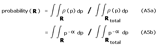 |
A specific example is considered - the probability that mean ("interpolated") prominence incorrectly misplaces gray area peaks with a 300 foot cutoff value and a 40 foot chart interval. The relevant regions, corresponding to R and Rtotal are shown in Figure A1.
R is the pair of yellow and blue triangles labeled A and B. By inspection each triangle occupies one-quarter of their prominence ranges - 280 to 300 feet and 300 to 320 feet, respectively. The remaining three-fourths of these ranges are labeled II and III and are colored light red.
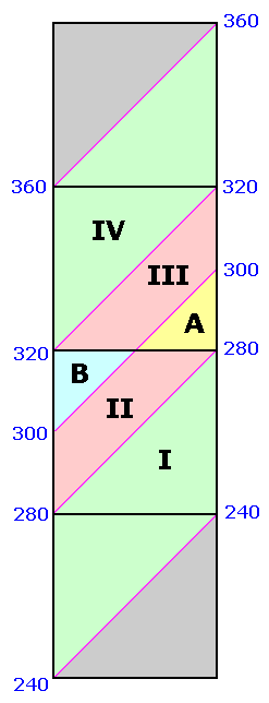
|
| Figure A1 |
Rtotal is the summed area of the middle two squares, and includes regions I, II, III and IV. Region I is one-half the 240 to 300 foot prominence range (green area within the second square from bottom). Region IV is one-half the 320 to 360 foot prominence range (green area within the second square from top).
Account must be made of these fractional contributions (as regions I through IV) of the various prominence intervals cited. These fractions are then included as a factors entering into the integrands of Equation (A5), and expressed as functions of the prominence p.
For yellow triangle A the fraction of region II occupied varies in a linear fashion from one-half at p = 300 feet to zero at p = 280 feet. By inspection the required integral is
 |
(A6a) |
where pcutoff is 300 feet. For blue triangle B the fraction of region III occupied varies linearly from one-half at p = 300 feet to zero at p = 320 feet. By inspection the required integral is
 |
(A6b) |
The numerator of Eqs.(A5a,b) is the sum of these two integrals. For the denominator there are four contributions, one from each of regions I through IV. Regions II and III contribute according to Eqs.(A5a) and (A5b), respectively, yet without the additional factors required to account for the fractional contributions of triangles A and B to these regions. For region II we have
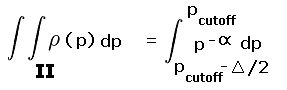 |
(A7a) |
while for region III,
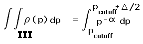 |
(A7b) |
Noting Figure A1, regions I and IV each occupy just one-half of their respective prominence ranges. Hence similar factors are required to evaluate their integrals just as with triangles A and B. Region I contains all (peak, saddle) pairs at p = 280 feet, diminishing linearly with prominence to no such pairs at p = 240 feet. Region IV contains all (peak, saddle) pairs at p = 320 feet, diminishing similarly to no pairs at p = 360 feet.
Correspondingly,
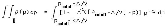 |
(A8a) |
while for region IV,
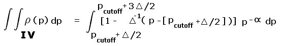 |
(A8b) |
The denominator of Eqs.(5a,b) is then the sum of the integrals on the right hand sides of Equations (7a, 7b, 8a, 8b).
Evaluation of these integrals is tedious to say the least. The integrand's exponential argument may,
depending on initial the choice of
assume the special value -1. In particular, = -2.0
results in some integrands containing the factor p-1.
When that occurs one replaces the elementary result for the integral
of xn, as xn+1/(n+1), by ln x.
The specific choice = 1.5 paired with
pcutoff = 300 feet and = 40 feet yields a
probability P = 0.12342, and is contrasted with the P = 0.125 result of
naively assuming that (x, y) is a constant.
For any region in (peak, saddle) space the mean prominence is
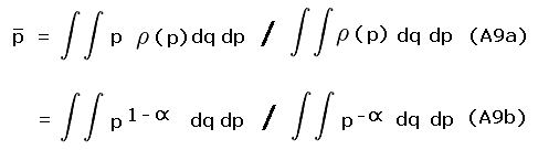 |
By "mean" we refer to the averaged prominence - NOT Pmean.
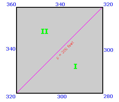
|
| Figure A2 |
A specific example is considered - mean prominence for the square in Figure A2 containing peaks from 280 to 360 feet of prominence. Significantly, the coordinate q enters, as it does with the probability calculation above, as a prominence-dependent factor describing what fraction of peaks, for a given p-value, lie within the region of interest.
By inspection we obtain for the triangle labeled I,
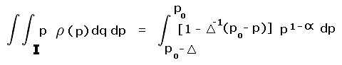 |
(A10a) |
while for triangle II,
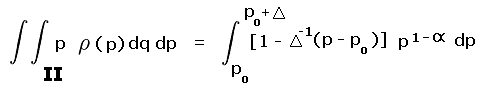 |
(A10b) |
In these equations po is the mean prominence assuming
(x, y) is a constant.
The numerator of Eqs.(A9a,b) is the sum of these two integrals. For the denominator we have the sum of Eqs.(A11a,b) -
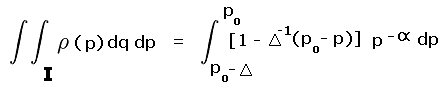 |
(A11a) |
while for triangle II,
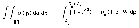 |
(A11b) |
These integrals are evaluated. Again, the integrand's exponential argument may,
depending on initial the choice of
assume the special value -1.
The specific choice = 1.5 is used, conforming more
closely to real data than other possible values for this exponent.
Together with po = 320 feet and = 40 feet
we obtain a mean prominence (in the term's statistical sense) of 318.755 feet.